
Quadruped Sim
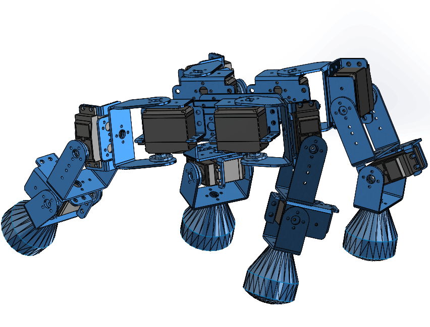
Much of this work is published in my PhD thesis.I designed in SolidWorks with parts that could be fabricated to real robots. The feet attachments were modified to be the shape of the physical sensors. The Solidworks file could be transferred over to URDF format which works with applications such as ROS and PyBullet.
Following previous successful work with CTRNNs (Continuous time recurrent neural networks), we use 6 fully connected neurons where two neurons are outputs to control the hip and knee motors for the quadruped, with the ankle motor constrained to simplify gait evolution. The ankle was positioned to face down 180 - knee_pos. This forced the robot to always be standing upright and reduced the necessary motor outputs to 2. For the Biped the two neurons control the ankle and hip. The CTRNN took a while to evolve oscillations, before even evolving gaits, therefore we introduced a sine output to enforce oscillations all the time. As debugging progressed, the CTRNN became an evolvable filter for the potential of sensory input. It would evolve output nodes that become parameters of the sine wave alongside a genotype encoded shift of phase, allowing legs to move in rhythmic sequences. Though this is not the conventional use of a CTRNN for gait evolution, our development of this model sped up the gait evolution and produced good gaits.
Environment conditions
To set different environments for the robots to adapt to, we first varied the frictional properties of the terrain. PyBullet allows changes in the lateral friction by setting a parameter so the frictions were set as follows (from low to high): 0.05, 0.10, 0.15, 0.20, 0.25, 0.30, 0.35, 0.40, 0.45, 0.50, 0.55, 0.60, 0.65, 0.70, 0.75, 0.80, 0.85, 0.90, and 0.95. These frictions were implemented on a flat surface, to single out the impact of friction on the gaits. However, we also wanted to test the effect of non-flat terrain. For this, we procedurally generated terrain with waves on the x- and y-axes and how curved or flat this wave is. The exact methods are outlined in this repository which is focussed on printable textures. Characteristics were chosen so they would be suitable for the experiments in the later chapter.Genetic Algorithm
We used various algorithms to optimize the gait controller which all use the same representation. All the algorithms optimised the parameters of the network plus the phase shifts\( x \sim \mathcal{U}(0, \text{num\_legs}) \)
Each gene is a float value, initially generated randomly from a Gaussian distribution of mean 0 and standard deviation 4, as well as with different maximum and minimum limits: -4 to 4 for the weights, -16 to 16 for the biases, and -1 and 1 for the oscillation offset $\omega$. $\tau$ is also included in the genotype and is enforced to be larger than $dt$. These values were taken from previous work on evolved CTRNNs (jakobi,1998). For a CTRNN of 6 neurons, we have 36 weights, 6 biases, 12 oscillation offsets and tau per neuron. Making the genotype contain 66 genes. Our randomly generated Gaussian values use a mean of 0 and standard deviation of 4 picked arbitrarily. Fitness functions for gait adaptation has taken many forms which greatly depend on the task. Key features of gait adaptation include deviation from target, stability and energy consumption. As well as the underlining aspect of a robot falling over being hugely penalised. Assessing the success of a gait can be fairly simply achieved. If the goal is to get as far as possible then we can have an accumulative distance, but if the line being straight is important then we must consider other factors. We explore a few different equations that take into consideration different aspects of the environment. Overall we care about distance and straightness of the line, but the way in which we enforce this can be over time, involving speeds and taking into consideration deviation of orientation.The simulation is 3D, thus has an x, y and z axis. The z-axis represents the height of the robot; if it has fallen, the z-axis will be much lower than the start position. The x and y axes represent various directions the robot can move. We can use the x, y, and z positions of the robot over time to calculate how well it is performing.
Initial fitness (denoted as function \( \xi \)) was calculated by the total distance on the x-axis, with deviations in the y and z axes subtracted. Start coordinates of the agent are denoted by variable \( S \) and \( E \) represents the end coordinates. This was designed to enforce walking in a straight line. The y and z reductions are given a weighting \( w \) of 10 to decrease their importance relative to the x-axis.
\[ \xi(S,E) = \left| S_x - E_x \right| - \frac{\sum_{A \in \{y,z\}} \left( \left| S_A - E_A \right| \right)}{w} \]
This fitness function is only concerned with ending up somewhere on the direct path rather than enforcing a straight-line trajectory throughout. It can lead to workable gaits but may be too simple to generate elegant solutions.
The next fitness function, denoted by \( \varrho \), calculates distance over time in an attempt to enforce behaviour that sticks to a straight line. The issue with \( \xi \) is that a robot can deviate during movement as long as it finishes in the correct position. The term \( \left| X_T - X_0 \right| \) calculates the overall distance gained by the agent with weighting \( \theta \) controlling its importance. Penalisation is applied for movement in the Y and Z directions. The key addition is the inclusion of velocity changes over time, encouraging smooth and consistent motion.
\[ \varrho (X,Y,Z,V) = \frac{\left| X_T - X_0 \right|}{\theta} - \frac{\sum_{t=0}^{T}(Y_t^2 + Z_t^2)}{w} - \frac{\sum_{t=1}^{T}\left| V_t - V_{t-1} \right|}{\gamma} \]
Another issue observed across various fitness functions is the robot spinning while remaining on the same axis. Orientation is therefore important for maintaining straight-line locomotion. Orientation penalisation is shown below, where orientation is denoted by \( \phi \) and its magnitude is calculated over all axes.
\[ \varpi (X,\phi) = \sum_{t=1}^{T} \left| X_T - X_{t-1} \right| + \frac{\sum_{t=1}^{T} \left( \sqrt{\phi_x^2 + \phi_y^2 + \phi_z^2} \right)}{w} \]
Results Summary
