Datalogging device

Posted 25/04/2026

This tutorial covers the creation of a data logging device. We will learn how to use a Raspberry Pi Pico, connect a gyroscope/accelerometer sensor and create a dataset tat can be used for machine learning classification.

Smart fitness watches use small sensors that detect movement in 3D space, and can make use of the movements to detect if you are walking, running, cycling etchttps://github.com/shepai/datalogger_education/. and how quickly you are doing this. They pair this with heart rate monitors to provide more health information. This is something known as "multimodal", where we combine various sensors which often improves model accuracy. We will be (on a simple scale) learning to implement our own data gathering device, so that we too can make models for classifying movement.

Device construction

You will need a Raspberry Pi Pico, a computer with USB connection and to download Thonny IDE.

Once you have all of these, you may need to reflash the Raspberry Pi Pico if it is new. To do this hold down the bootsel button and then connect the USB to the pico and computer. Be sure to keep the button pressed during this time. Once it is connected it should come up with the boot menu. Drag the most recent download of CircuitPython for Pico into the folder.

See this tutorial for more detail.

Once all set up you will need to upload the library dependencies to the board. The files can be found under /Circuitpython_Dependencies. Copy and paste the contents of this folder into lib/ on the pico. If there are compatibility issues with any of these libraries it might be because your CircuitPython flash is more up to date than these libraries. If so you will need to install the latest ones from here.

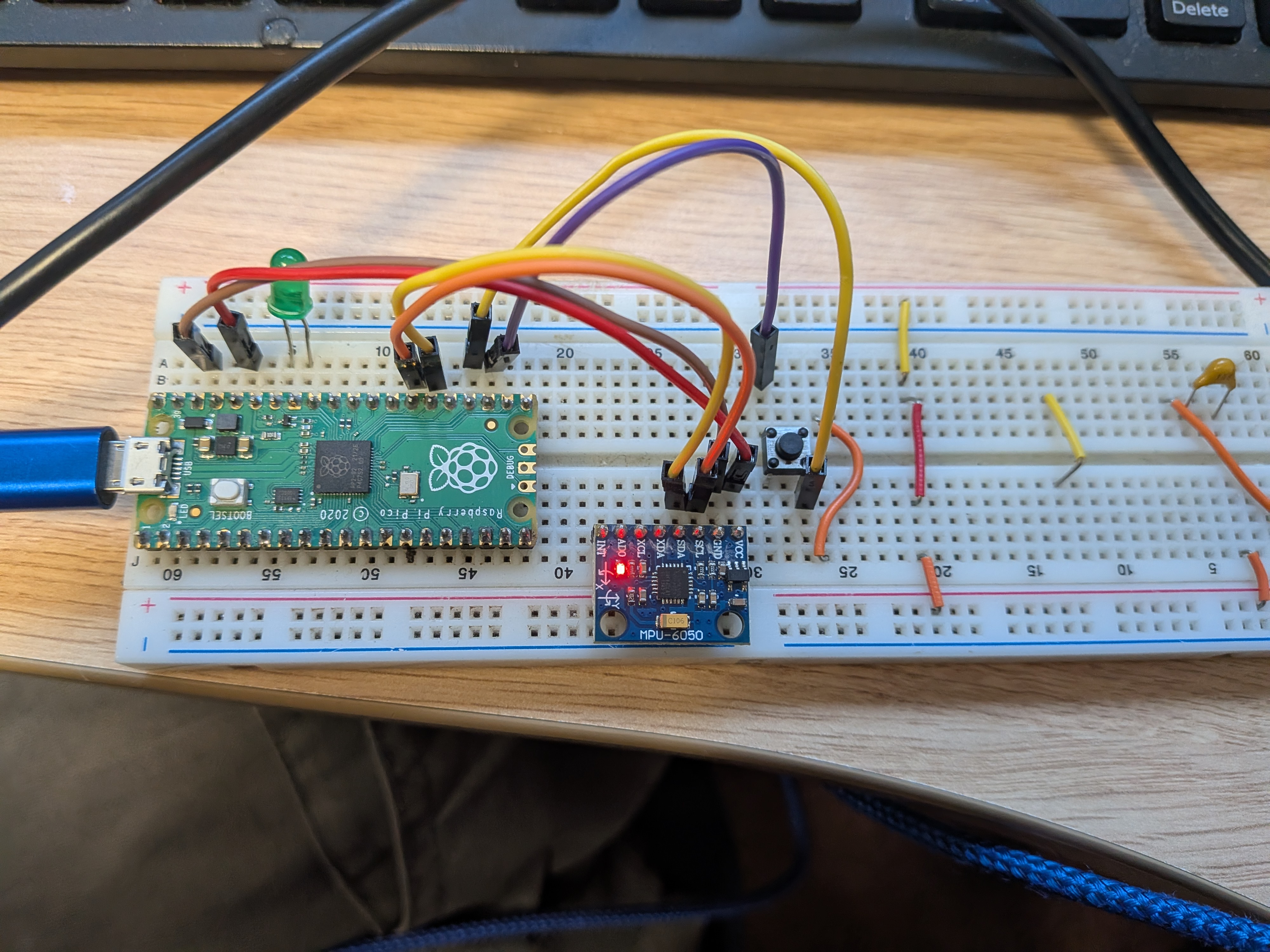
Wiring

To wire up your data logger you will need to select sensors you want to read from, SD card reader (optional), breadboard, buttons and Pico.

First begin by placing each component you will be using on the breadboard so that the lines do not cross, we will use jumper wires to connect the electronics.

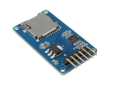
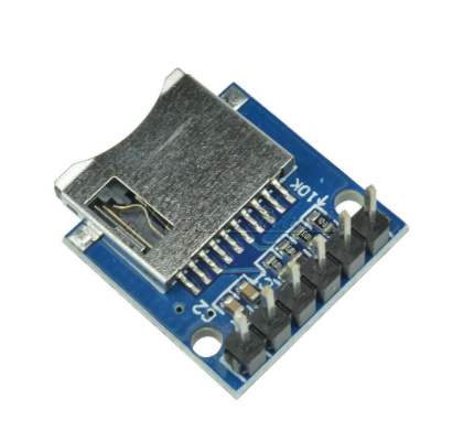
SD card

The SD card is optional, though if you do not use an SD card the device cannot be connected to Thonny while you gather data, otherwise you will get an error stating:

Traceback (most recent call last): File "<stdin>", 
line 48, in <module> File "<stdin>", 
line 20, in __init__ 
RuntimeError: Cannot remount path when visible via USB.

If this happens, simply unplug the device and make sure your code is running on boot by saving it as code.py. If using USB and it keeps reconnecting to Thonny, use a power bank and gather your dataset manually. Ideally in datalogging for larger datasets you would use some form of external storage, like an SD card, because it can store more data.

If you do have an SD card then it is wired as follows:

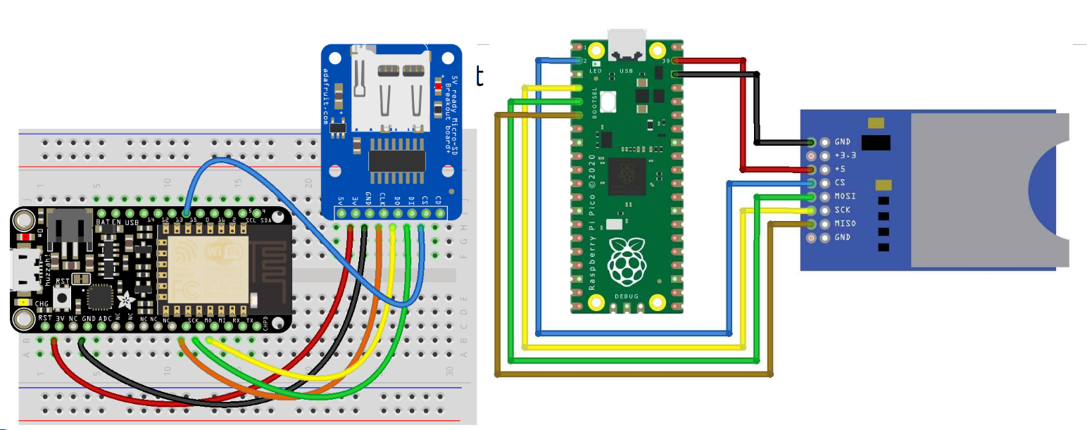
SD Pin	Pico Pin
MOSI	GP3
MISO	GP4
GND	GND
5V/3.3	See table below
SCK	GP2
CS	GP1

Different SD readers may have different power requirements:

SD card holder	Power requirement	Pin on Pico
	5V	VBUS
	3.3V	3.3

MPU6050 sensor

The MPU6050 is a gyroscope, accelerometer and temperature sensor. We will use it to gather human movement datasets.

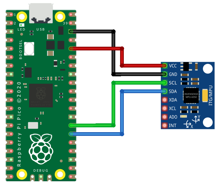
MPU6050 Pin	Pico Pin
GND	GND
VCC	3.3
SDA	GP20
SCL	GP21

Push button

We include a push button to allow you to stop and start recording.

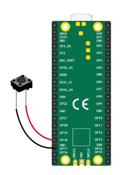
LED

The LED is our user interface. It indicates whether data is being recorded.

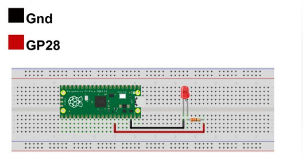
The longer pin is positive, shorter is negative. Connect the shorter pin to GND and the longer pin to GP28.

Coding

Once the libraries are uploaded under the lib folder, upload the demo code.py file to the pico and rename it to code.py so it runs on boot.

import busio
import digitalio
import board
from dataloggerCP import datalogger
import adafruit_mpu6050
import time

The program then sets up communication interfaces. SPI is configured for communicating with a data logger (likely an SD card), and I2C is set up to talk to the MPU6050 sensor.

spi = busio.SPI(board.GP2, board.GP3, board.GP4)
cs = board.GP1
i2c = busio.I2C(board.GP21, board.GP20)

A button is configured as an input with a pull-up resistor. This means the button reads True when not pressed and False when pressed. An LED is also configured as an output to indicate whether recording is active.

btn = digitalio.DigitalInOut(board.GP18)
btn.direction = digitalio.Direction.INPUT
btn.pull = digitalio.Pull.UP

LED = digitalio.DigitalInOut(board.GP28)
LED.direction = digitalio.Direction.OUTPUT

The MPU6050 sensor and the data logger are then initialized.

mpu = adafruit_mpu6050.MPU6050(i2c)
logger = datalogger(spi, cs)

A function called read() is defined. This function collects acceleration and gyroscope data from the sensor, converts the values into strings, and formats them as a comma-separated line suitable for saving in a CSV file.

def read():
    xa, ya, za = mpu.acceleration
    xg, yg, zg = mpu.gyro
    return str(xa)+","+str(ya)+","+str(za)+","
    +str(xg)+","+str(yg)+","+str(zg)+"\n"

Some variables are initialized to control the program state. The toggle variable determines whether recording is active, the LED is initially turned off, and num is used to create unique filenames.

toggle = False
LED.value = False
num = 0

The main loop runs continuously. Inside the loop, the program checks if the button is pressed. Because of the pull-up configuration, a pressed button is detected when btn.value is False. When pressed, the recording state is toggled and the LED changes state.

while 1:
    if not btn.value:
        toggle = not toggle
        LED.value = not LED.value

If a file is currently open, it is closed to stop recording. If no file is open, a new CSV file is created with a name like log0.csv, log1.csv, and so on.

        if logger.opened:
            logger.close()
        else:
            logger.create_file("log" + str(num) + ".csv")
            num += 1

A short delay is added to prevent multiple rapid button presses from being registered.

        time.sleep(0.2)

If recording is active, the program reads a line of sensor data and writes it to the file.

    if toggle:
        dataline = read()
        logger.write_data(dataline)

Another short delay controls how frequently data is recorded.

    time.sleep(0.1)

Overall, the system works as a simple data logger. Pressing the button starts recording motion data to a new file and turns the LED on. Pressing the button again stops recording and turns the LED off.

Gathering your dataset

Now you have a device that can record multiple datasets. When powered, it is ready. Press the button to start recording (LED on), press again to stop.

Files will be saved as log0.csv, log1.csv, etc. Keep track of what each file represents for later classification.

Ideally, use an external phone charger to power the device on the move. Otherwise, keep it connected to your laptop and carefully perform tasks while holding the device. Try to keep recordings similar length.

Machine Learning

This part of the tutorial focuses on classifying our datasets. If you haven't managed to download data, we have an example dataset in the repository to make use of.

The first step in building a machine learning model from sensor data is loading the recorded files into a usable format. Each file contains raw motion data collected from the device, where each row represents a moment in time and contains acceleration and gyroscope readings across three axes. Since the CSV files do not include column names, these are manually assigned after loading so the data can be accessed more clearly.

You should use your data you gathered to load in.

df = pd.read_csv("demos/1/walking.csv", header=None)
df.columns = ["ax", "ay", "az", "gx", "gy", "gz"]
df.head()

Once loaded, the data can be visualised to understand its structure and behaviour over time. Plotting the acceleration and gyroscope signals helps reveal patterns such as periodic motion, noise, or differences between activities. This step is important because it gives an intuition for what the model will later try to learn.

plt.plot(df['ax'], label="x-axis")
plt.plot(df['ay'], label="y-axis")
plt.plot(df['az'], label="z-axis")
plt.title("Acceleration over time")
plt.legend()
plt.show()

plt.plot(df['gx'], label="x-axis")
plt.plot(df['gy'], label="y-axis")
plt.plot(df['gz'], label="z-axis")
plt.title("Gyroscope over time")
plt.legend()
plt.show()

To train a model, multiple recordings are needed, each representing a different class of behaviour. These files are grouped together along with labels that describe what action is being performed. For example, walking, running, and idle might each correspond to different motion patterns. These lists allow the program to systematically load all data and associate each sequence with the correct label.

files = ["demos/1/walking.csv",
    "demos/1/running.csv",
    "demos/1/idle.csv"]
labels = ["walking","running","idle"]

The data from these files is then converted into a format suitable for machine learning. Instead of treating each row independently, the data is grouped into sequences over time, forming a large time-series dataset. This is essential because motion is not defined by a single reading, but by how readings change over time. A function such as convert_data typically performs this step by stacking windows of data together and aligning them with their labels.

To learn from this type of sequential data, a Long Short-Term Memory (LSTM) network is used. An LSTM is a type of neural network designed specifically for time-series data. Unlike standard neural networks that treat inputs independently, LSTMs maintain a memory of previous inputs, allowing them to recognise patterns that unfold over time. This makes them well suited for motion data, where the difference between actions like walking and running lies in the rhythm and progression of movement rather than individual values.

The model is constructed using stacked LSTM layers. The first layer processes the full sequence and passes its output to the next layer, allowing the network to build increasingly complex representations of the motion. Dropout layers are included to reduce overfitting by randomly disabling parts of the network during training. Finally, dense layers convert the learned representation into a prediction over the possible classes.

n_timesteps = X_data.shape[1]
n_channels  = X_data.shape[2]
n_classes   = len(np.unique(y_data))

model = Sequential([
    LSTM(64, return_sequences=True, 
    input_shape=(n_timesteps, n_channels)),
    Dropout(0.3),

    LSTM(64),
    Dropout(0.3),

    Dense(32, activation="relu"),
    Dense(n_classes, activation="softmax")
])

model.compile(
    optimizer=Adam(1e-3),
    loss="sparse_categorical_crossentropy",
    metrics=["accuracy"]
)

model.summary()

Once defined, the model is trained using the collected dataset. During training, the network adjusts its internal parameters to minimise the difference between its predictions and the true labels. This process is repeated over multiple epochs, gradually improving performance.

history = model.fit(
    X_data, y_data,
    epochs=10,
    batch_size=32,
    validation_split=0,
    shuffle=True
)

loss, acc = model.evaluate(X_data, y_data, verbose=0)
print("Model Accuracy:", acc*100,"%")

After training, it is important to evaluate how well the model is performing. A confusion matrix provides a detailed view of this by showing how often each class is correctly or incorrectly predicted. This helps identify specific weaknesses, such as one activity being confused with another.

from sklearn.metrics import confusion_matrix
from sklearn.metrics import ConfusionMatrixDisplay
from sklearn.metrics import accuracy_score

y_pred_probs = model.predict(X_data)
y_pred = np.argmax(y_pred_probs, axis=1)

cm = confusion_matrix(y_data, y_pred)
disp = ConfusionMatrixDisplay(cm)
disp.plot()
plt.show()

Overall, this pipeline transforms raw sensor readings into a trained model capable of recognising patterns in motion. The key idea is that the LSTM learns temporal relationships in the data, allowing it to distinguish between different activities based on how the signals evolve over time rather than just their instantaneous values.