Bio-Inspired Navigation for Varied Terrain

This project investigates the use of evolutionary approaches to enable robotic agents to learn their own physical limitations in a visual navigation task. Within nature, biological agents understand their own limitations when it comes to crossing complex terrain. By attempting to cross terrain that an agent is not built for they risk injury or even death. A robot needs to understand its own limitation if it is to be able to explore complex terrain but not get damaged. One applications of this would be planetary exploration where robot damage would ruin a cost expensive mission. The project was split into three parts: Navigation; vision; and the development of the physical robot.
Navigation strategies were developed in a two-dimensional simulation world with procedurally generated terrain. Simulation takes less time to trial than physical experiments, therefore a proof of concept could be developed within the time constraints of this project. Environmental hazards were introduced, such as water, and experimentation into hyper-parameters and algorithm choice allowed convergence on high fitness models. Agents learned to follow contours in order to minimize energy consumption and avoid hazardous environments.
Two depth sensors were trialled for visual base navigation. One was using two cameras and the OpenCV disparity function; the other an off-the-shelf approach with the Xbox Kinect. Stereo imaging was picked as it best highlighted the environmental attributes that would be relevant for solving the problem of hazardous terrain representation. The Kinect sensor was the best at finding depth. Further processing took place to squeeze the depth images into a compressed representation that could be used in the simulated trained agent model.
The physical robot made use of the visual depth information and neural networks trained in simu- lation trials which were able to cross the bridge between simulation and the real world (known as the ‘reality gap’). It could predict hazardous terrain for avoidance in an outdoor environment. The chassis was inspired by how cockroaches cross obstacles, it used Whegs and a bendable back to improve movement over rocky and outdoor environments. Whegs are a hybrid between wheels and legs where the cyclic efficiency of the wheel is used, but claw features are added to improve climb like a leg. The back bending control was learned by the system using a population of hillclimbers evolving the weights and biases of a neural model. This project successfully demonstrated that an agent can understand its hazardous environment, and learn to overcome obstacles.

Simulation

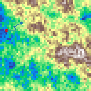
I set up the simulated environment illustrated in the below figure using Python by generating a 2D map from Perlin noise. Perlin noise is a type of gradient noise commonly used to procedurally generate terrain [21] where the value of the space between two points changes smoothly. A grid of n dimensions is created and each position is assigned a random vector, where the dot product is calculated between the gradient vector and the offset vector. This allows interpolation between each dot product to generate noise within the grid.

In such simulations, we can find how far a point is from the start position and the terrain steepness (gradient) at any point. The energy consumed (E) by a robot in a given trial is calculated from the number of steps taken (S) and the accumulated terrain value of each place (P). Each position on the map has a value that represents how high or low the ground is. Very low values would be submerged underwater and high values be at the top of the mountains. The difference between movement is the step S up, down, or across from the current height. This is called the terrain value. More energy is used going uphill than downhill, so these state transitions are valuable for calculating fitness. The Manhattan distance is used as a measure of how far the agent has travelled. This was picked in place of the Euclidean distance as the 2D terrain guarantees a worst case scenario. Euclidean distance finds the shortest path, which may not be the best path.
The agent was written as its own class, where on initialisation the network structure could be determined. Weights and biases are generated when an array of Gaussian noise is entered through the set genes method as a parameter. Using a forward function, the network uses PyTorch and generates output that is converted to a vector choice using the argmax function. There are eight directions that the agent can take, therefore the network is expected to generate the probabilities of a success of each vector. The success for this method is seen in the figure where the agent has navigated through the terrain. The vector of movement allowed the agent to traverse across the environment.

Physical robot

The initial Wheg design would get caught while reversing as the claws were only grabbing one way and the robot also struggled to turn left and right on the spot. The addition of a tilting mechanisms for left and right turns was added to solve this. In some circumstances, when the robot would try to climb, it would need an element of height to get over obstacles. This was achieved by adding a stabiliser servo with a wheel caster on the bottom. When deployed, the wheel caster allowed the robot to carry on moving without getting caught. The heavy battery was placed at the back of the robot as it was discovered that the front needed to be lighter than the back to have improved climbing abilities.
The robot made use of an off the shelf kinect sensor. This is better calibrated than a homemade stereo vision sensor, although the kinext sensor is much larger and mounting it on the robot would require a more powerful battery and a larger chassis. Therefore, this camera will only be used as a proof of concept for using depth navigation in a real world environment.

For vision-based navigation, the robot made use of a depth camera. The Xbox Kinect was used to gather depth imaging of the environment. This was reduced in scale to 5 by 5 pixels to highlight key features about the terrain. Using this image, the trained agent within the simulation was deployed to use a convolutional neural network. This was because the Conv2D network architecture had the best accuracy within the given trials.
As there are multiple directions that can be valid within these examples, using numeric based validation methods was not possible without mass labelling the data. This would still be down to human judgement. Instead, human judgement over the examples will be the evaluation method of how well the model performed in the real world. The network was trained to predict a vector of movement out of eight possible moves, but as this was not controlling the robot, so the vector is simply displayed as the chosen direction of travel that should be taken.
Evolving this navigation model directly on the robot could lead to better results. This is because the model will learn how its own hardware and control deals with different sized obstacles, and which obstacles the chassis could overcome with back-bending. This method was not used because enforcing reward posed too many challenges. Knowing when the robot has collided, got stuck and used energy requires a number of sensors. Additionally, it would have taken a large amount of time to perform just one trial. Simulation mostly converged on peak fitness at generation 400 to 800. Additionally, if the simulated model performs well it will have shown the model to be robust enough to cross the reality gap between simulation and physical implementation.
The reduction of the image to a 5 x 5 pixels input for the model was applied to both depth images. One generated by the Kinect and one generated by the OpenCV disparity function from two USB webcams. Based on my previous results, both used the area interpolation resizing method.

Results

Evaluation of how the simulated trained model reacts to the real world robot vision is denoted by the following qualitative examples. These show the original image, how the depth sensor views this, how the robot views this and the direction the model predicts. The vector is in the direction of movement of the line triangular marker. The unmarked end is the start position of the vector. This terrain in the Figure above is deemed too hazardous by the model, where the vector tells the agent to turn sharply left. This is considered a success case.